Gamma Correction and Image Smoothing with OpenCV
Understand gamma correction and explore various image smoothing techniques using OpenCV and Python, with practical code examples and visualizations.
🌈 Understanding Gamma Correction
Gamma correction is a key concept in digital imaging and display systems. It helps align how brightness is captured, stored, and displayed with how the human eye perceives it.
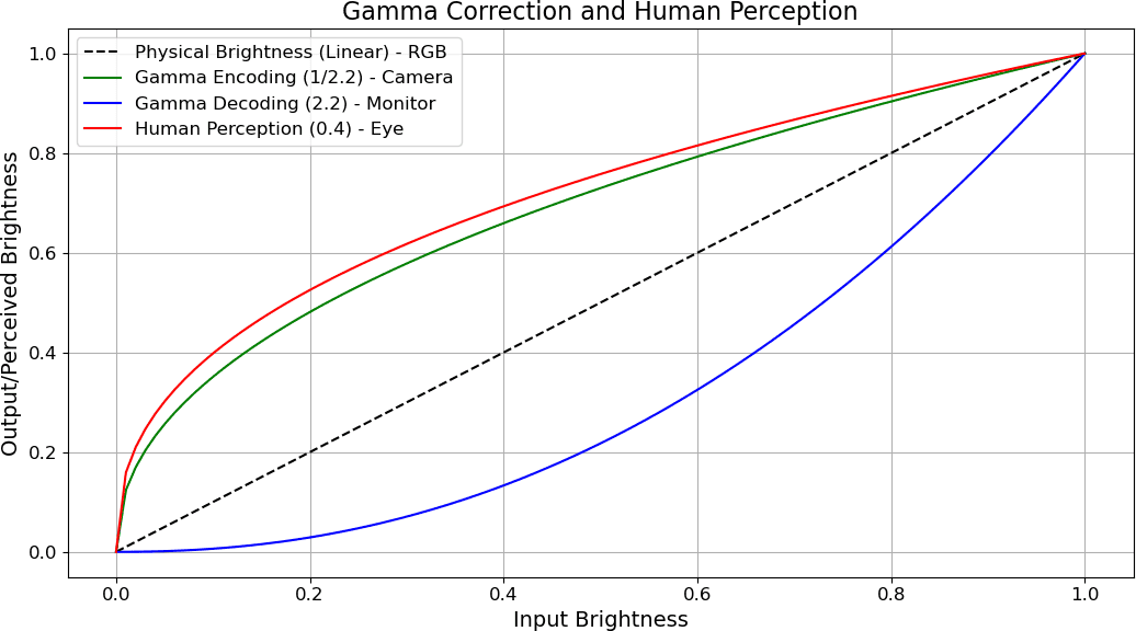
This graph shows the relationship between input brightness (X-axis) and output or perceived brightness (Y-axis) through various gamma curves.
Linear Brightness — Dashed Line
- The black dashed line represents physical brightness increasing linearly.
- Example: If brightness =
0.5, the light is 50% of max. - But our eyes don’t perceive brightness linearly.
👁 Human Perception — Red Curve (γ ≈ 0.4)
- The red line represents how the human eye perceives brightness.
- We are more sensitive to dark tones than bright ones.
- Linear brightness of
0.5feels closer to~0.7in perceived brightness. - Our eyes boost shadows naturally.
📷 Gamma Encoding — Green Curve (γ = 1/2.2 ≈ 0.45)
- Cameras apply gamma encoding to images before storing them.
- This curve compresses highlights and expands shadows.
- Why?
- Human eyes detect more detail in shadows.
- Encoding this way makes better use of limited bit depth (like 8-bit RGB).
- Gamma encoding makes stored image more eye-friendly.
🖥 Gamma Decoding — Blue Curve (γ = 2.2)
- Monitors apply gamma correction (decoding) to the image before display.
- This reverses the encoding, using a gamma of ~2.2.
- Without this, the image would look too dark.
✅ Final Effect: Linear Perception
- The combination of encoding (
γ ≈ 0.45) and decoding (γ ≈ 2.2) brings the brightness back to a linear perceptual experience. - This ensures what we see matches the original scene realistically.
📌 Summary
| Concept | Gamma Value | Purpose |
|---|---|---|
| Linear RGB | 1.0 | Physical light intensity |
| Human Perception | 0.4 | Eye is more sensitive to darks |
| Camera Encoding | 1/2.2 | Stores image closer to human vision |
| Monitor Correction | 2.2 | Adjusts for display/human mismatch |
Want to see a live demo or code implementation in Python or OpenCV? Let me know!
Prerequisites
You'll need the following Python libraries:
- opencv-python: For image processing operations
- matplotlib: For displaying images
- numpy: For numerical operations
Install them with:
pip install opencv-python matplotlib numpy
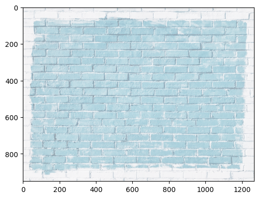
Step 1: Reading and Displaying an Image
Let's start by reading an image as RGB and normalizing its values between 0 and 1:
def readRGB(imageName):
    img = cv2.imread('Assets/' + imageName).astype(np.float32) / 255
    img = cv2.cvtColor(img, cv2.COLOR_BGR2RGB)
    return img

def show(img):
    fig = plt.figure(figsize=(6,6))
    ax = fig.add_subplot(111)
    ax.imshow(img)
    plt.show()

image = readRGB('bricks.jpg')
show(image)

Step 2: Gamma Correction
Gamma correction adjusts the brightness of an image. A higher gamma value darkens the image, while a lower gamma value brightens it.
gamma = 1/4
result = np.power(image, gamma)
show(result)
Note: Gamma correction is essential for displaying images correctly on different screens and for certain image processing tasks.
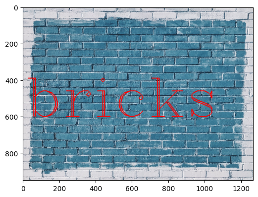
Step 3: Adding Text to an Image
You can add text to an image using OpenCV's putText function:
font = cv2.FONT_HERSHEY_COMPLEX
cv2.putText(image, text='bricks', org=(10,600), fontFace=font, fontScale=10, color=(255,0,0), thickness=4, lineType=cv2.LINE_AA)
show(image)
Step 4: Image Smoothing (Blurring)
Smoothing is used to reduce noise and detail in images. There are several common techniques:
1. Custom Kernel Convolution
kernel = np.ones(shape=(5,5), dtype=np.float32) / 25
destination = cv2.filter2D(image, -1, kernel)
show(destination)
Explanation:
The codekernel = np.ones(shape=(5,5), dtype=np.float32) / 25creates a 5x5 matrix (kernel) where every element is1/25 = 0.04. This kernel is used for image smoothing (blurring) by averaging the pixel values in a 5x5 neighborhood.The line
destination = cv2.filter2D(image, -1, kernel)applies this kernel to the image using convolution. Here, the-1argument tells OpenCV to use the same depth (number of bits per pixel) for the output image as the input image. In other words,-1means "keep the original image's data type." This function replaces each pixel's value with the average of its surrounding 25 pixels (the 5x5 neighborhood), resulting in a simple uniform blur effect. The result is stored in thedestinationvariable, which contains the smoothed (blurred) image.

2. Averaging (cv2.blur)
blur = cv2.blur(image, ksize=(5,5))
show(blur)
Explanation:
The functioncv2.blur(image, ksize=(5,5))applies a simple averaging filter to the image. It works by sliding a 5x5 window (kernel) over the image and replacing each pixel value with the average of all the pixel values inside that window. This process smooths the image by reducing sharp transitions and noise, resulting in a blurred effect. The larger the kernel size, the stronger the blurring effect.

3. Gaussian Blur
gaussian = cv2.GaussianBlur(image, ksize=(15, 15), sigmaX=0)
show(gaussian)
Explanation:
What is Gaussian Blur?
Gaussian blur is a popular image smoothing technique that reduces noise and detail in an image. It works by averaging pixel values with their neighbors, but instead of giving each neighbor equal weight, it uses a bell-shaped (Gaussian) curve to give more importance to pixels closer to the center.How does it work?
- The algorithm uses a Gaussian kernel (a small matrix of numbers shaped by the Gaussian function) to determine how much each neighboring pixel should contribute to the new value of the center pixel.
- The kernel is slid over the image, and for each pixel, a weighted sum of its neighbors is calculated. Pixels closer to the center have higher weights.

Mathematical Formula:
The value of the Gaussian kernel at position (x, y) is:G(x, y) = (1 / (2πσ²)) * exp(-(x² + y²) / (2σ²))
- Here,
σ(sigma) controls how much the blur spreads out. A larger sigma means a blurrier image.- The kernel is normalized so that all its values add up to 1.
In Practice:
- For each pixel, the new value is a weighted average of its neighbors, with weights given by the Gaussian kernel.
- This process is called convolution.
- Both grayscale and color images can be blurred this way.
Effect:
- Gaussian blur is especially good at reducing random noise (like graininess) in images.
- The amount of blur depends on the kernel size and the sigma value (
sigmaXin OpenCV).- The result is a smoother, less noisy image, where sharp edges and details are softened.
4. Median Blur
Median blur is especially effective for reducing salt-and-pepper noise.
How does it work?
Consider an image corrupted with salt-and-pepper noise (random black and white pixels). When you apply median blur, a small window (kernel) slides over the image. For each position, the pixel values inside the kernel are collected, and the median value (the middle value when sorted) is found. The center pixel is then replaced with this median. This process removes isolated outlier pixels (like salt and pepper noise) while preserving edges better than averaging filters, because the median is less affected by extreme values.
median = cv2.medianBlur(image, 5)
show(median)

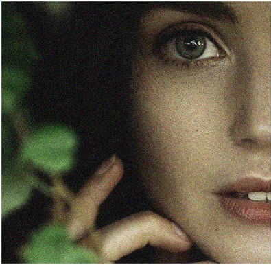
Step 5: Real-World Example – Noise Reduction
Let's see how median blur can reduce noise in a real-world image:
woman_image = readRGB('noise_woman.png')
show(woman_image)

reducedNoiseImage = cv2.medianBlur(woman_image, 3)
show(reducedNoiseImage)

Step 6: Bilateral Filtering
Bilateral filtering is a powerful technique for noise removal that stands out because it preserves sharp edges in the image, unlike other smoothing filters. While filters like Gaussian blur use a spatial Gaussian function to average nearby pixels (regardless of their intensity), this can cause edges to become blurred, since the filter does not distinguish between pixels of similar or different intensities.
Bilateral filtering improves on this by combining two Gaussian functions: one that considers the spatial closeness of pixels (like Gaussian blur), and another that considers the similarity in pixel intensity. This means that only nearby pixels with similar intensity values to the central pixel contribute significantly to the blur. As a result, edges—where there is a large intensity difference—are preserved, and only similar, nearby pixels are averaged together. This makes bilateral filtering highly effective for noise reduction while keeping edges sharp. However, this operation is computationally more intensive and slower compared to simpler filters like Gaussian or median blur.
bilateral = cv2.bilateralFilter(image, d=9, sigmaColor=75, sigmaSpace=75)
show(bilateral)

Parameters:
d: Diameter of each pixel neighborhood.sigmaColor: This controls how much the filter considers differences in color or intensity between pixels. A higher value means that pixels with more different colors can still influence each other, so the filter will blur across bigger color differences. A lower value means only pixels with very similar colors will be averaged together.sigmaSpace: This controls how far away (in terms of distance in the image) pixels can be and still influence each other. A larger value means that pixels farther apart can affect each other, leading to a smoother, more blended result. A smaller value means only very close pixels are considered, so the effect is more local.