Introduction to Image Processing with OpenCV

Overview

Image processing is a fundamental concept in computer vision and artificial intelligence. In this tutorial, we'll explore basic image processing operations using OpenCV, a powerful library for computer vision tasks.

Prerequisites

Before starting, make sure you have the following libraries installed:

To follow along with this tutorial, you'll need to install three Python libraries:

• opencv-python: This is the Python binding for OpenCV, a powerful library for image processing and computer vision tasks.
• matplotlib: A popular library for plotting and visualizing data, which we'll use to display images.
• numpy: A fundamental package for numerical computations in Python, used for handling arrays and matrices, which are essential in image processing.

You can install all of them using the following command:

Basic Setup

Let's start by importing the necessary libraries:

import cv2
from matplotlib import pyplot as plt
import numpy as np

Step 1: Reading and Displaying Images

Reading an Image

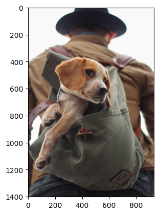
The first step in image processing is to read an image from your file system:

# Read the image
img = cv2.imread('Assets/dog_backpack.jpg')

Converting Color Space

OpenCV reads images in BGR (Blue, Green, Red) format by default, but matplotlib expects RGB format. We need to convert the color space:

# Convert the image from BGR to RGB
img_rgb = cv2.cvtColor(img, cv2.COLOR_BGR2RGB)

Displaying the Image

Now we can display the image using matplotlib:

# Display the image in RGB Mode
plt.imshow(img_rgb)
plt.show()

Step 2: Image Manipulation

Flipping Images

One common image manipulation is flipping. Let's flip the image vertically (upside down):

# Flip the image upside down (vertically) and display it
img_flip = cv2.flip(img_rgb, 0)
plt.imshow(img_flip)
plt.show()

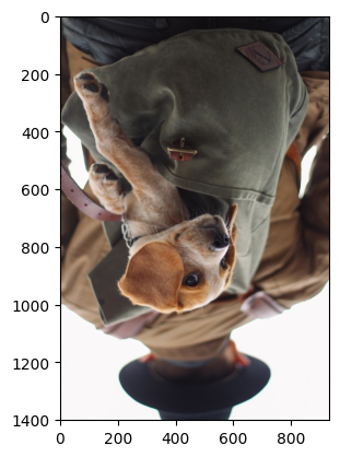
Understanding the flip parameter:

• 0: Flip vertically (upside down)
• 1: Flip horizontally (left to right)
• -1: Flip both vertically and horizontally

Step 3: Drawing on Images

Drawing Rectangles

OpenCV provides functions to draw various shapes on images. Let's draw a red rectangle around the dog's face:

# Draw an empty RED rectangle around the dogs face and display the image
cv2.rectangle(img_rgb, pt1=(200, 380), pt2=(600, 700), color=(255, 0, 0), thickness=10)
plt.imshow(img_rgb)
plt.show()

Parameters explained:

• pt1=(200, 380): Top-left corner coordinates (x, y)
• pt2=(600, 700): Bottom-right corner coordinates (x, y)
• color=(255, 0, 0): RGB color (Red in this case)
• thickness=10: Line thickness in pixels

Drawing Polygons

We can also draw more complex shapes like triangles:

# Draw a BLUE TRIANGLE in the middle of the image and display the image
pts = np.array([[250, 700], [425, 400], [600, 700]], dtype=np.int32)
cv2.polylines(img_rgb, [pts], isClosed=True, color=(0, 0, 255), thickness=10)
plt.imshow(img_rgb)
plt.show()

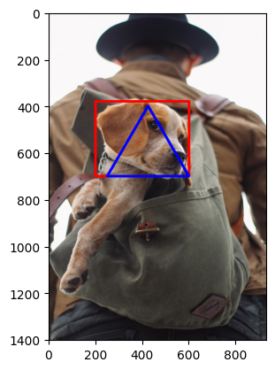
Understanding the parameters:

• pts: Array of points defining the polygon vertices
• isClosed=True: Connects the last point to the first point
• color=(0, 0, 255): Blue color in RGB format
• thickness=10: Line thickness

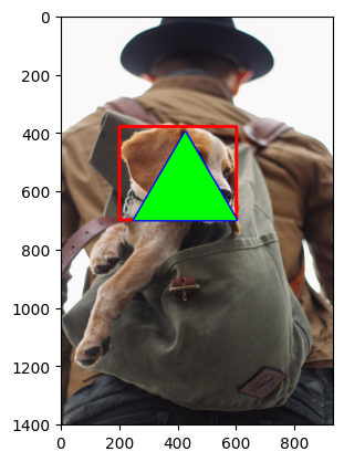
Filling Polygons

We can fill polygons with color using cv2.fillPoly():

# Fill the triangle with GREEN color and display image
cv2.fillPoly(img_rgb, [pts], color=(0, 255, 0))
plt.imshow(img_rgb)
plt.show()

Key Concepts Explained

Color Spaces

BGR vs RGB:

• OpenCV uses BGR (Blue, Green, Red) color space
• Most other libraries (matplotlib, PIL) use RGB
• Always convert when switching between libraries

Coordinate System

Image Coordinates:

• Origin (0,0) is at the top-left corner
• X-axis increases from left to right
• Y-axis increases from top to bottom

Color Values

RGB Color Format:

• Each color channel ranges from 0 to 255
• (255, 0, 0): Pure Red
• (0, 255, 0): Pure Green
• (0, 0, 255): Pure Blue
• (0, 0, 0): Black
• (255, 255, 255): White

Common Image Processing Operations

1. Image Reading and Display

# Read image
img = cv2.imread('image.jpg')
# Convert BGR to RGB
img_rgb = cv2.cvtColor(img, cv2.COLOR_BGR2RGB)
# Display
plt.imshow(img_rgb)
plt.show()

2. Image Flipping

# Vertical flip
img_flip_v = cv2.flip(img, 0)
# Horizontal flip
img_flip_h = cv2.flip(img, 1)

3. Drawing Shapes

# Rectangle
cv2.rectangle(img, (x1, y1), (x2, y2), (255, 0, 0), thickness)
# Circle
cv2.circle(img, (x, y), radius, (0, 255, 0), thickness)
# Line
cv2.line(img, (x1, y1), (x2, y2), (0, 0, 255), thickness)

Complete Code Example

Here's the complete code from this tutorial:

import cv2
from matplotlib import pyplot as plt
import numpy as np

# Read the image
img = cv2.imread('Assets/dog_backpack.jpg')

# Convert the image from BGR to RGB
img_rgb = cv2.cvtColor(img, cv2.COLOR_BGR2RGB)

# Display the image in RGB Mode
plt.imshow(img_rgb)
plt.show()

# Flip the image upside down (vertically) and display it
img_flip = cv2.flip(img_rgb, 0)
plt.imshow(img_flip)
plt.show()

# Draw an empty RED rectangle around the dogs face and display the image
cv2.rectangle(img_rgb, pt1=(200, 380), pt2=(600, 700), color=(255, 0, 0), thickness=10)
plt.imshow(img_rgb)
plt.show()

# Draw a BLUE TRIANGLE in the middle of the image and display the image
pts = np.array([[250, 700], [425, 400], [600, 700]], dtype=np.int32)
cv2.polylines(img_rgb, [pts], isClosed=True, color=(0, 0, 255), thickness=10)
plt.imshow(img_rgb)
plt.show()

# Fill the triangle with GREEN color and display image
cv2.fillPoly(img_rgb, [pts], color=(0, 255, 0))
plt.imshow(img_rgb)
plt.show()